Non-Technical Introduction to Our Bitcoin Modeling Framework

In this blog, I want to explain the basic structure of the Bitcoin price analysis framework and develop a single model as an example of how it works in practice. Now that the updated framework is fully functional, I want to 'take it out for a spin.'

Frameworks and Models

In a past journal article, we developed a Bitcoin price modeling framework and, in a recent working paper, updated it.

To clarify, a 'framework' provides the scaffolding for developing various 'models' that can be used to test particular theories and hypotheses. While I have yet to get into hypothesis testing, that is where I am heading after the framework is fully developed and the variables are credibily parameterized.

In a prior post, I outlined supply and demand fundamentals, and how they shape the development of this framework. Give it a read if you are unfamiliar with the basics of supply and demand analysis.

Building a Model

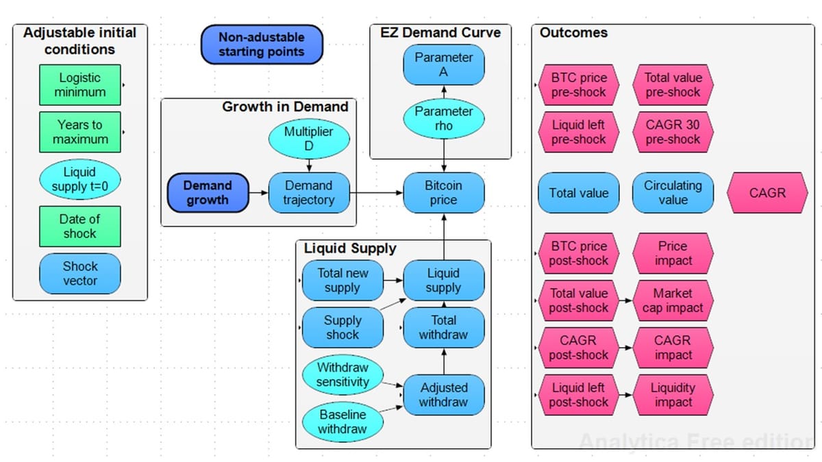
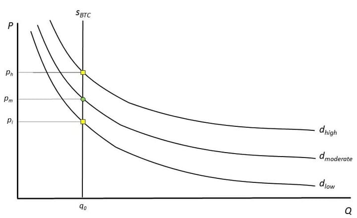
Three factors affect Bitcoin price: a demand curve that accounts for the intertemporal preferences of different kinds of investors ('traders' and 'HODLers'); a multiplier that accounts for external drivers of demand (adoption, macro factors); and liquid supply. All three form the core of this framework:

The framework allows for customizing the functional form and choices of parameters for each price determinant.

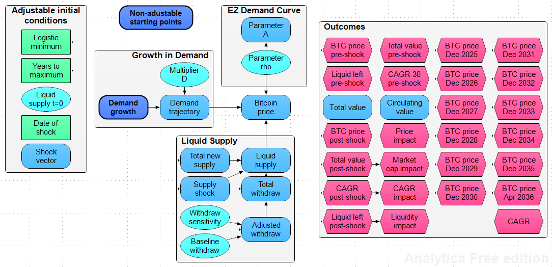
In the chart above, the turquoise ovals are variables that are continuous and uncertain: their functional form and parameters can easily be changed. The green rectangles are choice variables that give a limited number of discrete options for a parameter. Light blue rounded rectangles are intermediate variables that are calculated by the model; and the magenta hexagons are various model outputs of potential interest. To keep things relatively clean, the dark blue rounded rectangles just hide some of the intermediate variables.

You'll notice - and this is different from the working paper - that I have built in a number of new outcome variables. Most of them are for quickly pulling prices for specific milestones, as well as assessing the day-before to day-after impact of supply and demand shocks.

Model Constants and Variables

Pre-Set Starting Points

• Start date: April 21, 2024 (4th halving)
• End date: April 16, 2036 (anticipated date of the 7th halving)
• Start date price: $64,858
• Start date circulating supply: 19,687,500 Bitcoin
• Assumed inaccessible Bitcoin in all Satoshi wallets: 968,000
• Assumed inaccessible Bitcoin in all lost wallets: 1.57 million
• Daily emissions from Bitcoin mining: currently 3.125 Bitcoin/block (450/day), declinining by half for each of the 5th and 6th epochs

Flexible Starting Points

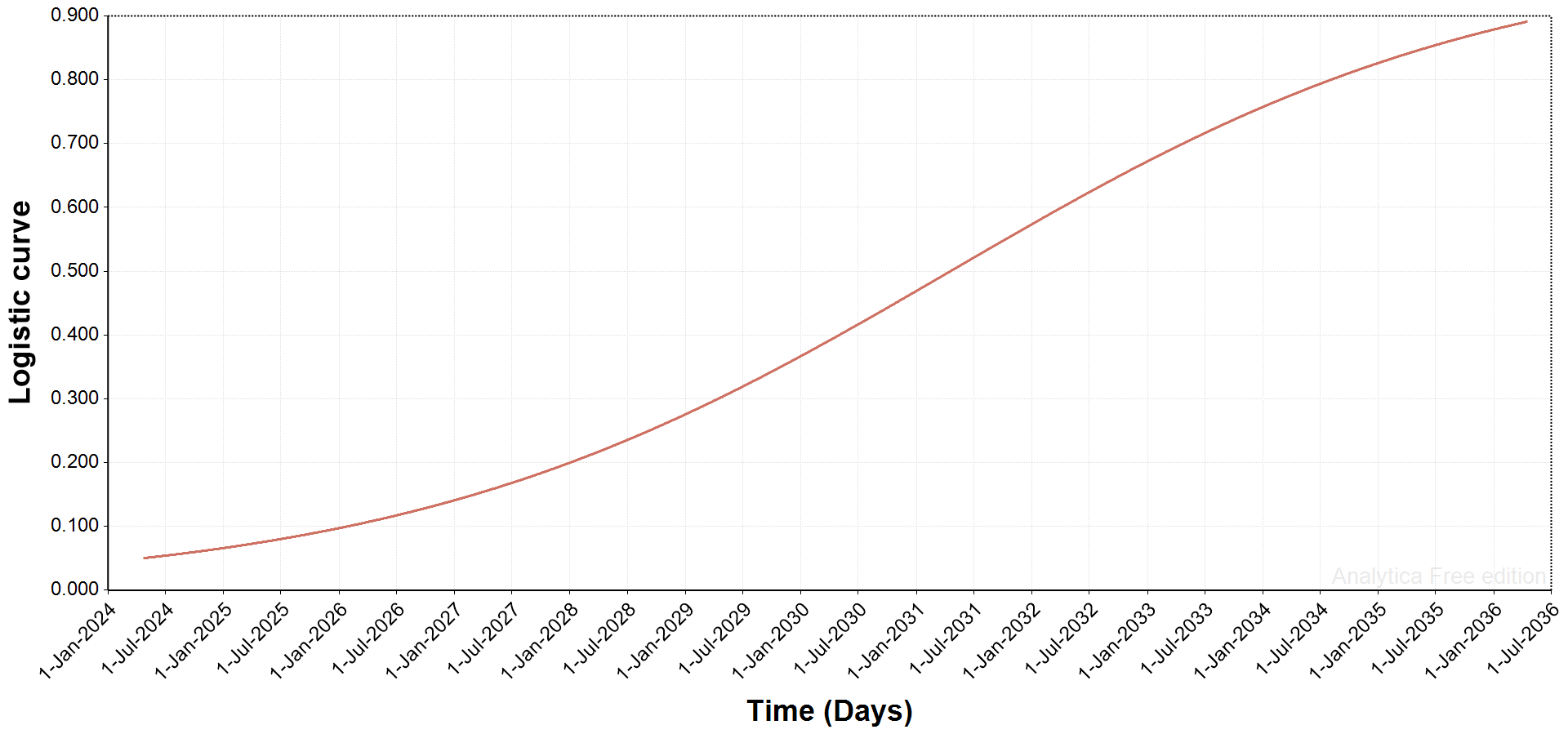
• Logistic minimum = choice of 0.01 to 0.08, in 0.01 increments. This variable describes how early we are in the Bitcoin technological adoption curve and feeds into growth in demand over time. The lower the value, the earlier we are, and the more pronounced the S-shaped adoption curve.
• Years to maximum = 6 to 16 years, in 2 year increments. This is the time until the adoption curve hits its saturation point: by default in a logistic function, the inflection point is midway between 0 and the chosen number of years.
• Date of shock is an optional date for testing specific demand or supply shocks.
• In the working paper, and in the example below, I used 0.05 as the logistic minimum and a 14 year period to saturation. This gives a fairly conservative adoption curve where inflection is noticable but not rapid, as would be seen in with more aggressive logistic curve parameters:

Growth in Demand

In this framework, I use a demand multiplier that feeds into the Bitcoin price. The inputs here are the logistic adoption curve (above), the value of the multiplier parameter, A, from the Epstein-Zin demand curve, and a demand multiplier, D, which is chosen from a range.

With the Epstein-Zin demand curve, A is fixed once the intertemporal tradeoff variable, rho, is chosen (more on that below).

The multiplier D, which reflects the external level of demand for Bitcoin (think macro variables here), helps calibrate the model, bringing predicted prices in line with forecast prices early in the model (see the working paper for more on this).

As we move forward in time, it makes sense that new sources of demand will come online for Bitcoin - MicroStrategy's moves to develop Bitcoin-backed alternatives to traditional bonds are one good example. The level of demand is not merely dependent on network effects in a traditional technological adoption sense, an impact of a growing network of users, but also macro and regulatory factors that stimulate additional, new types of investment and investment at scale.

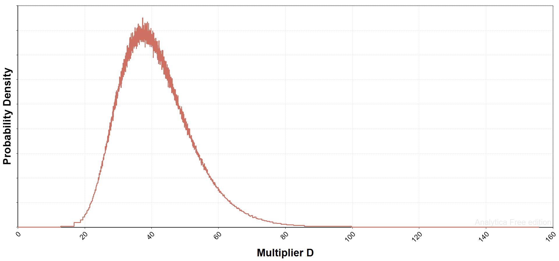
There is a lot of uncertainty regarding future demand, so it is appropriate to our variable D an uncertain probability distribution. In the working paper, we used a uniform distribution, which implied random selection between a specified lower and upper bound.

But any kind of distribution, if warranted, can be used. For example, here is a lognormal distribution (median 40, geometric standard deviation 1.3) that I use below, showing the distribution of 10,000 drawn Monte Carlo samples. You can see we get a few draws below 20 and a skinny upper tail, a key characteristic of lognormal distributions, that extends well beyond 80.

Epstein-Zin Demand Function

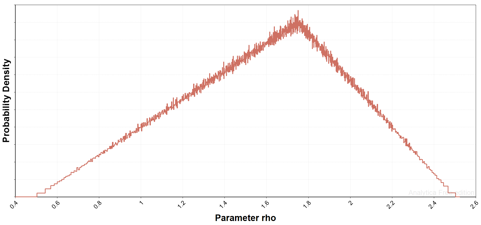
The EZ demand function is interesting because it accounts for intertemporal substitution. For Bitcoiners, this is pretty easy to understand: choosing the parameter rho determines time preferences. Low rho investors are traders with a high time preference; high rho investors are HODLers in it for the long haul despite price volatility.

The recursive EZ function is quite complex (see the working paper) but under certain assumptions, which seen quite plausible for Bitcoin investing, existing wealth level and a risk parameter drop out of the first-order conditions. This is really handy because it allows us to focus solely on how HODLing versus trading directly impacts liquid supply and price forecasts.

In the working paper, I had discrete choice options for rho, ranging from 0.50 (traders) to 2.5 (HODLers). In the example below, I instead used a triangular distribution function: my rationale here was that current investors probably lean towards HODLing. It was unclear if there was any particular functional form that would be most appropriate, so I thought it best to pick from a range with an upward, but uncertain, skew.

Liquid Supply

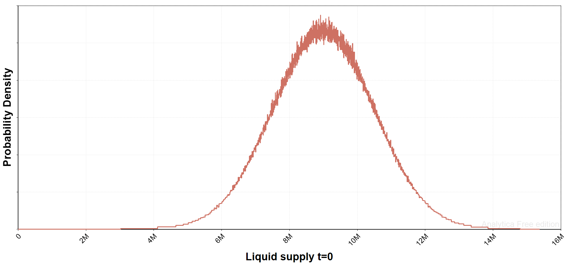
There are a few things to consider regarding liquid supply. First - and most importantly - what were the initial conditions at the start of the model's time horizon? While I used a uniform distribution between 5 and 13 million in the working paper, here I use a normal distribution with a mean of 9 million (same midpoint) and standard deviation of 1.5 million. This will reduce the number of fairly extreme outliers relative to the uniform distribution.

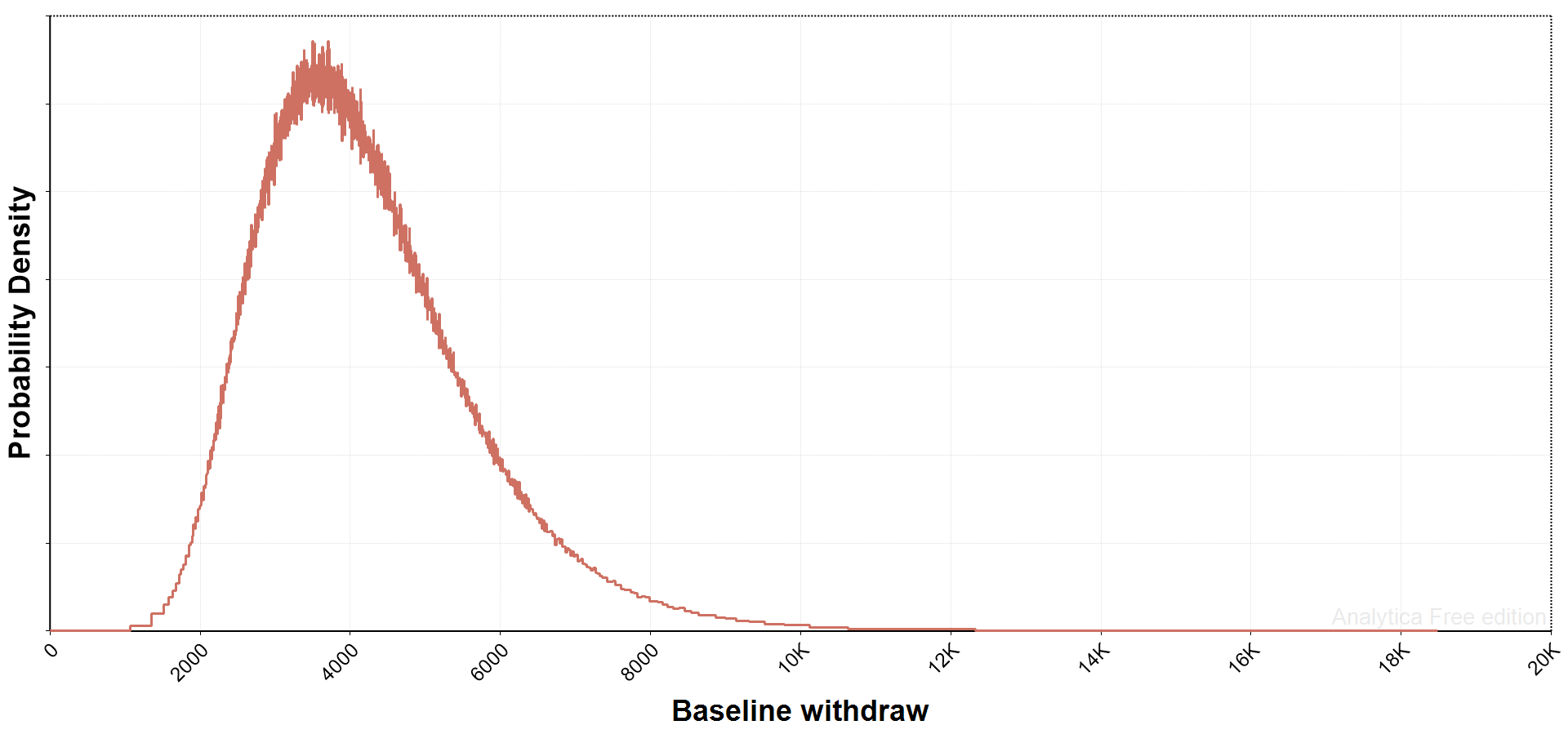
Next, there is a need to make assumptions about how many Bitcoin are removed from liquid supply each day. In the working paper, I drew from a uniform distribution between 1000 and 8000 per day. In this example, I instead use another lognormal distribution (median=4000, geometric mean=1.4), which gives a few outliers below 2,000 and above 8,000 per day.

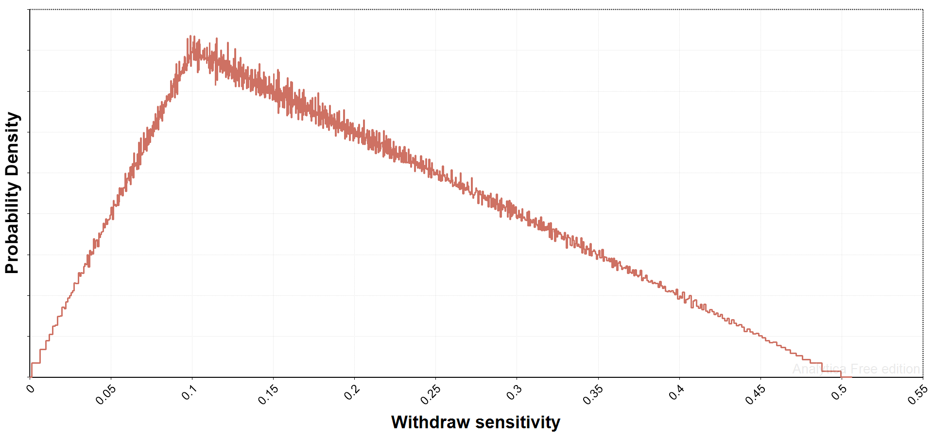
Finally, I have a new withdrawal elasticity parameter in the working paper. One of the obvious shortcomings in the journal publication was that buyers kept drawing the same amount of Bitcoin from liquid supply every day, no matter how high the price of Bitcoin had gone. The new parameter throttles the number of Bitcoin withdrawn on a daily basis, slowing Bitcoin demand as price appreciates. At the lowest level, the effect is quite subtle; at higher levels, it tends to throttle back new buying relatively quickly when price rises steeply.

Other factors may influence this parameter as well, relating to the ease of accessing Bitcoin via exchanges or OTC desks, and some other factors. This parameter can really be thought of as one that affects disciplined trade execution. In the working paper I had a uniform distribution over a full range of possibilities; below, I instead use another triangular distribution (maximum frequency at 0.10):

Supply Shock

Finally, the last new feature in the framework is its ability to incorporate either supply or demand shocks at particular dates. In this example, I use a simple example: on December 31, 2025, a single buyer comes into the market and makes a purchase, above and beyond normal daily removals (median=4,000 per day), of 500,000 Bitcoin.

Model Implementation

Because numerous variables are defined as continuous functions, I use Monte Carlo simulations to estimate price, liquidity, and other outcomes. 'Monte Carlo' comes from the game, where you spin the wheel and land a number. In modeling, it means that you 'spin the wheel' and draw a possible value from the feasible range of values for each uncertain variable in the model. This is a way to sample the entire space of possible outcomes, including those that common and those that are rare.

I use 10,000 draws (median Latin hypercube sampling) for each model run.

The parameter choices below are a pretty fair reflection on my own personal thinking at the moment - I haven't hit the run button yet for the new simulation as I write this. So, now, for you and I, let's see how this particular model of Bitcoin prcie trajectory formation takes us.

Results

Liquid Supply Forecast

The 500,000 block purchase at the end of 2026 is clear in the supply forecast.

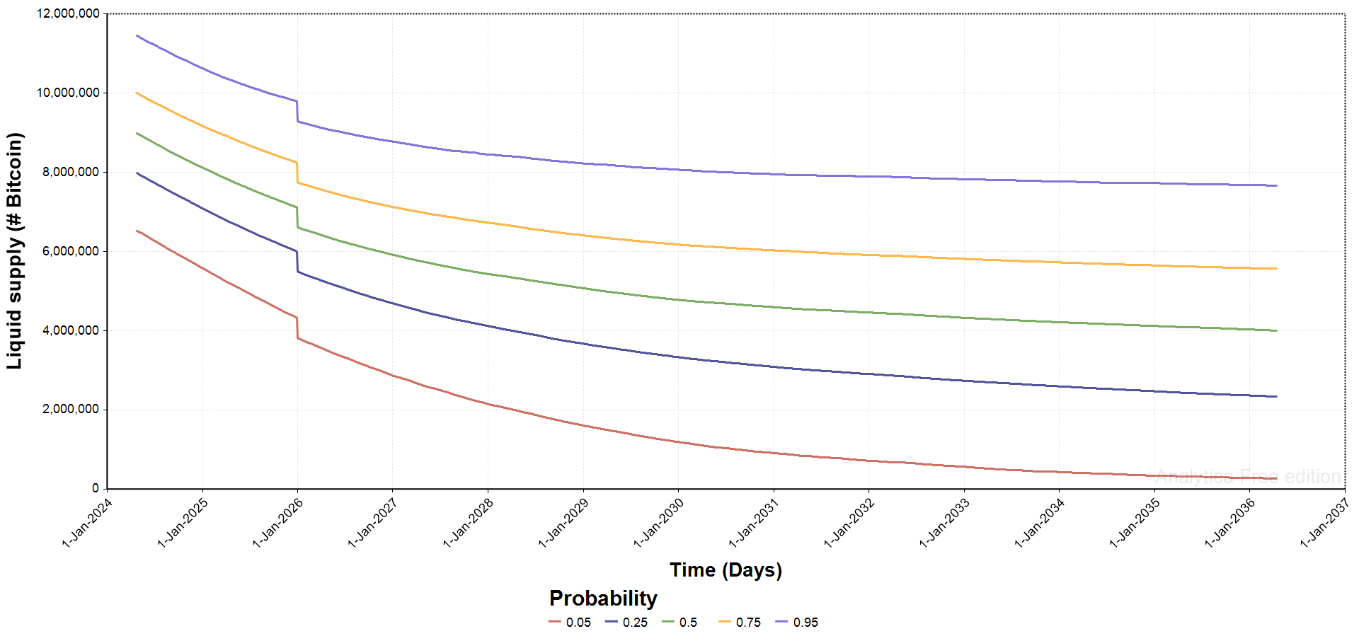
The chart shows median (center line) projected liquid supply and the two upper and lower bands are confidence intervals. Right away, see how the 95% band dips under 2 million liquid supply by mid-2027: this is an obvious flag (from prior papers) that a full-on supply shock and hyperbolic price increase is still a possibility, even taking fairly conservative approach parameter assumptions in this model.

That lower band reaches the 2-million threshold early, with the 500,000 withdrawal from liquid supply in late-2026 accelerating the timeline slightly. However, it is clear that the supply would have breached that level later even without this shock of a surprise 500,000 Bitcoin purchase.

Other bands flatten out over time, likely showing some residual impact from the Dec 2026 withdrawal but, at first glance, there is nothing that obviously hints at eventual price instability.

Bitcoin Price Trajectory

As expected, based on those low liquid Bitcoin levels for the 95% band, hyperbolic price increases are a non-trivial outcome in this model. That shows up in the figure below. For the 40% band, the final price forecast is $4.36 million in April 2036. Down at the 5% band, the forecast price is still $2.52 million by April 2036 (higher than the $1.98 million in the working paper).

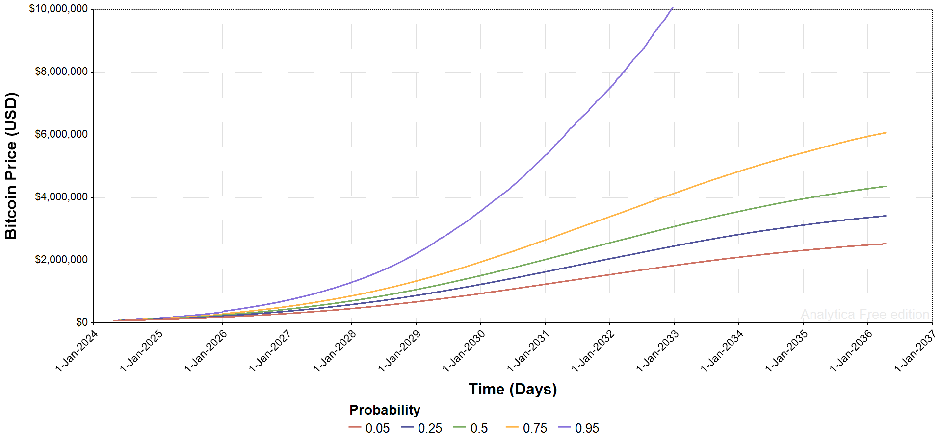
It is easy now easy to pull price forecasts for any particular day over the time horizon (want to know what Bitcoin price is forecast for your birthday in 2032?). For instance, here are the projections, by probability band, for December 31, 2026:

• 5% - $293,668
• 25% - $366,988
• 50% - $431,506
• 75% - $515,330
• 95% - $714,517

It's also easy to pull the dates that each band hits a particular price milestone. Here are the dates for $1 million per Bitcoin, taking account of that big buy at the end of 2026:

• 95% - July 22, 2027
• 75 % - May 5, 2028
• 50 % - Nov 10, 2028
• 25% - May 22, 2028
• 5% - Mar 30, 2030

Market Cap

Market capitalization (based on circulating Bitcoin) shows a similar pattern, running from $52.5 to $126.5 trillion for the four non-hyperbolic probability bands.

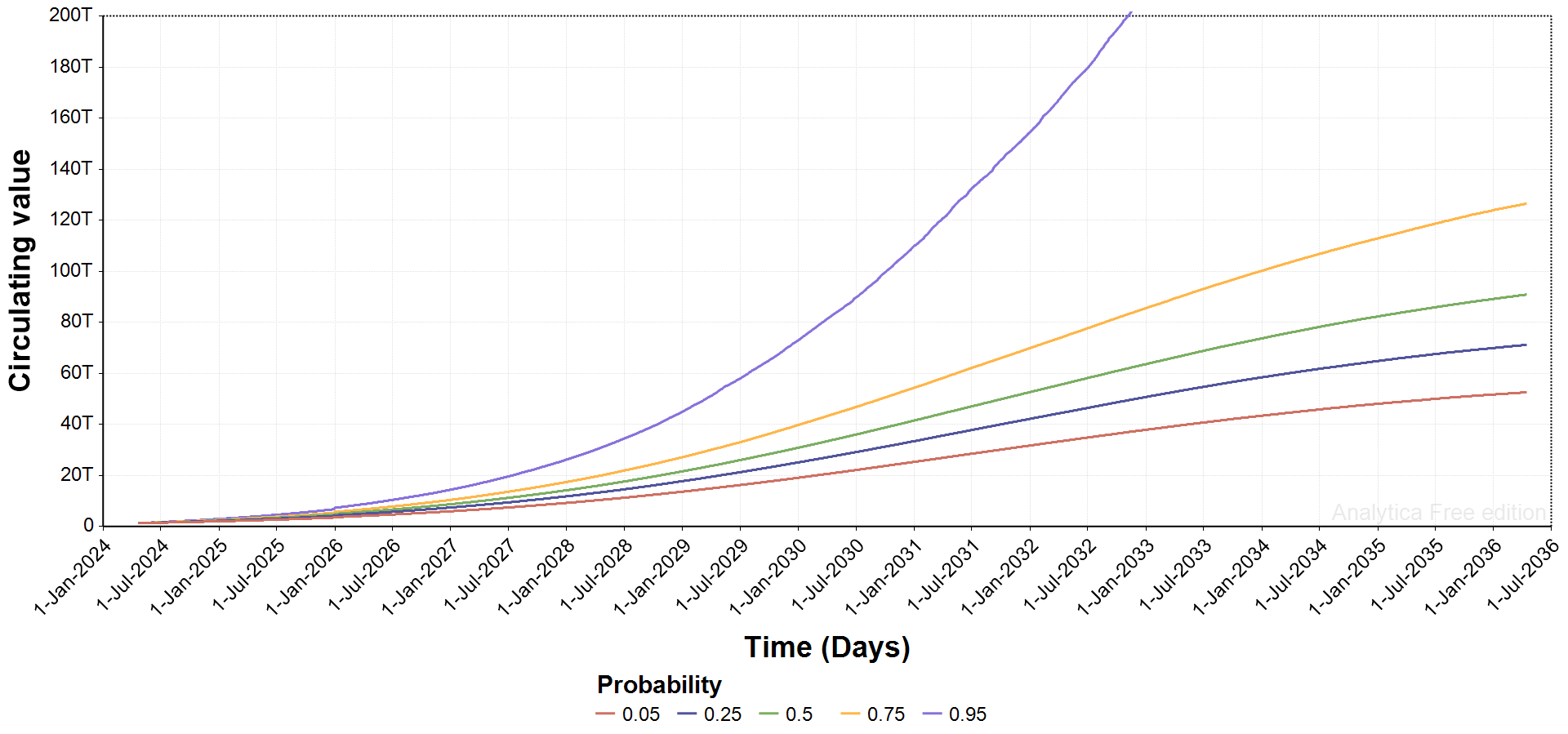
Some astronomical USD prices out in the tails make for nonsensical market cap in the 95% band. Well, I shouldn't say nonsensical, because there actually is a perfectly good explanation: the US $ collapses in purchasing power and it no longer makes sense to price things in a radically debased American dollar.

This model is saying that there's >5% odds of hyperbolic price appreciation happening by the early-2030s. But remember, we do not have paper Bitcoin and derivatives built into the framework (yet), so those may lower the odds and/or slow the advent of any coming collapse (but adding counterparty risk that could blow up).

Supply Shock

Finally, let's look at the impact of the 500,000 Bitcoin buy on December 31, 2026. The immediate price impact of the reduction of supply by 500,000 above and beyond normal removals (median = 4,000 per day) has pretty modest price impact. It ranges from $6,084 for the 5% band up to $11,680 for the 50% band, and $31,862 for the 95% band.

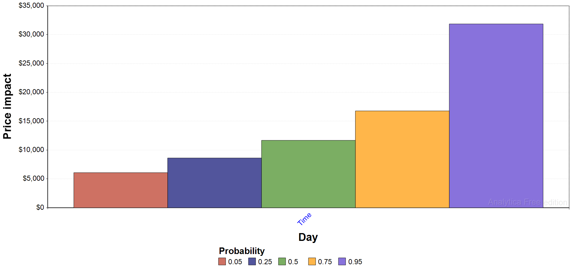
The supply-side impact is modest when there is lots of liquid supply but, out in the tail, where starting liquid supply would be lowest, you see disproportionate price increases.

Bitcoin market price the day prior (December 30) to the big buy range from $172,587 for the 5% band, up to $232,726 for the median, and up to $336,373 for the 95% band, so percentage increases were 3.5%, 5.0%, and 9.5%, respectively.

While I haven't yet run models for later supply shocks, one would expect to see more of those 5- or 6-figure price movements as supply gets scarce (I covered this in the current working paper).

I have not factored in a demand-side shock in this analysis, it is likely substantial. Thnk of a big, publicly-announced Bitcoin purchase by a sovereign wealth fund: it would certainly be the case that the demand multiplier, D, would jump sharply. The demand side FOMO would probably far outweigh the actual impact from the change in supply itself, at least when liquid supply has not yet been depleted to the 2-3 million Bitcoin lelel.

Model insights

Modeling Messages

As in our working paper, I think the messages from this model, with its more constrained functional forms, reinforces prior findings:

• Multi-million dollar Bitcoin prices are to be expected;
• Market cap gets up to the $100+ trillion range without hyperbolic price appreciation and the subsequent collapse of the US dollar;
• Supply-side shocks have relatively minor impact until liquid supply is running very thin.

Some Speculations

• We can start to infer how much liquid supply is really out there from real-world market reactions to supply inflows and outflows. A few weeks ago, we had a whale move 80,000 Bitcoin to Galaxy, and dump the whole bag over the course of a few hours. That had surprisingly little impact on price, which suggests there's still may be substantial liquid supply in the market.
• Demand side shocks are likely much more common given market psychology, and investors' being prone to panic over every piece of bad news and euphoric when good news comes out. To me, this says that market volatility is primarily a demand-side issue at the current time (and it can be modeled).
• Having finished the prior papers and now testing even more new models, I am getting the feeling that the core results are probably pretty robust, with significant price appreciation being the norm, and with some hyperbolic price increasese still possible. This will take more testing, however, to nail down, especially given the impacts of large volumes of paper Bitcoin in the market.

Next Steps

I have a few directions I would like to take this framework going forward:

1. Develop an open-source web-based model that anyone can play with
2. Start to incorporate 'paper Bitcoin' into the model: synthetic exposure and derivatives functionally bend the vertical supply curve right around market price, providing a way to 'cheat' a little regarding Bitcoin's absolute fixed supply limits. I think it would be valuable to try to figure out how to incorporate this, so we can better understand
   1. the impact on real Bitcoin withdrawals to cold storage and pressure on liquid supply;
   2. the implications for price trajectory and momentum (how much does paper Bitcoin availability slow price appreciation?);
   3. the possibilities for increased volatility should paper Bitcoin trades fall apart in the face of real supply depletion of real Bitcoin; and
   4. how derivatives and synthetic exposure can be used, in conjunction with policies targeting withdrawal sensitivity, to control hyperbolic price increases arising from far right tail events.
3. Tie in corporate and national treasury strategies, to assess their potential impact on liquid supply and Bitcoin price forecasts (and vice versa, the impact of different possible Bitcoin price trajectories on treasury company viability)
4. Start to integrate macro price determinants in the market demand multiplier, which could lead to better shorter-term price forecasts that really capture the gyrations of market demand's implact on price determination.

Take a close look at the assumptions I used above. It would be great to get some perspectives on whether people think these are reasonable. With reasonable assumptions, the credibility level of the forecast outputs rises.