Exploring Bitcoin's Price Trajectory: An Interactive Supply-Demand Model

How high could Bitcoin's price go – and what drives it there? This interactive tool lets you explore one answer to that question by adjusting the key economic assumptions behind a peer-reviewed supply-demand model of Bitcoin price formation.

The modeling app is available here:

The model replicates our Analytica code used in the original research paper: Rudd, Murray A. and Dennis Porter 2025. Bitcoin supply, demand, and price dynamics. Journal of Risk and Financial Management 18: 570. doi: https://doi.org/10.3390/jrfm18100570

It also draws on an earlier paper that first developed the approach: Rudd, Murray A. and Dennis Porter 2025. A supply and demand framework for Bitcoin price forecasting. Journal of Risk and Financial Management 18: 66. doi: https://doi.org/10.3390/jrfm18020066

Those are technical reads - I'd suggest playing around with the model using Table 8 in the first paper, and then tweak model variables from there. Probably most importantly, the tool allows you to enter your own assumptions about lost and illiquid Bitcoin.

What this model does

This model forecasts Bitcoin's price trajectory from April 2024 (the 4th halving) through April 2036 (the 7th halving) using fundamental economic principles rather than historical price patterns or statistical extrapolation. At its core, the model calculates a daily equilibrium price by intersecting Bitcoin's perfectly inelastic (vertical) supply curve with a demand curve that grows over time according to a logistic adoption path.

The key insight: Bitcoin is the only globally traded asset with a mathematically guaranteed hard cap on supply. When demand grows against a fixed and shrinking liquid supply, price must adjust. And the adjustment can be dramatic.

Note that, at the moment, I have only implemented a deterministic model. The Bitcoin supply, demand, and price dynamics article also contains a Monte Carlo model: I will post this in the future.

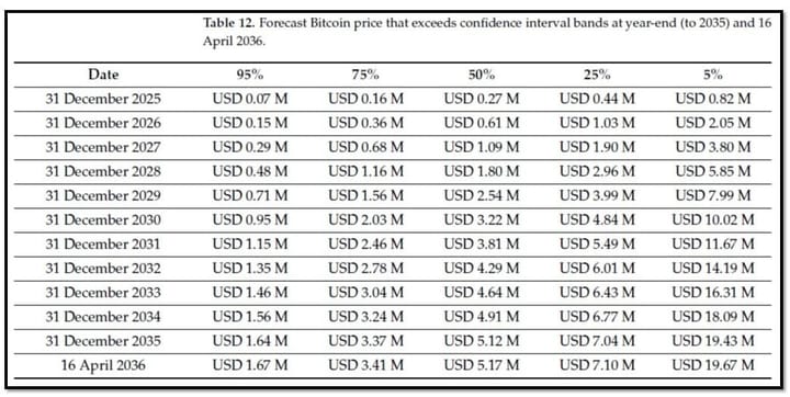
In the Monte Carlo implementation in our paper, we just ran the deterministic model 10,000 times with randomly drawn parameters for every variable. Pay attention to Table 12 in the paper - that's the real take-home of this modeling effort.

The economic framework

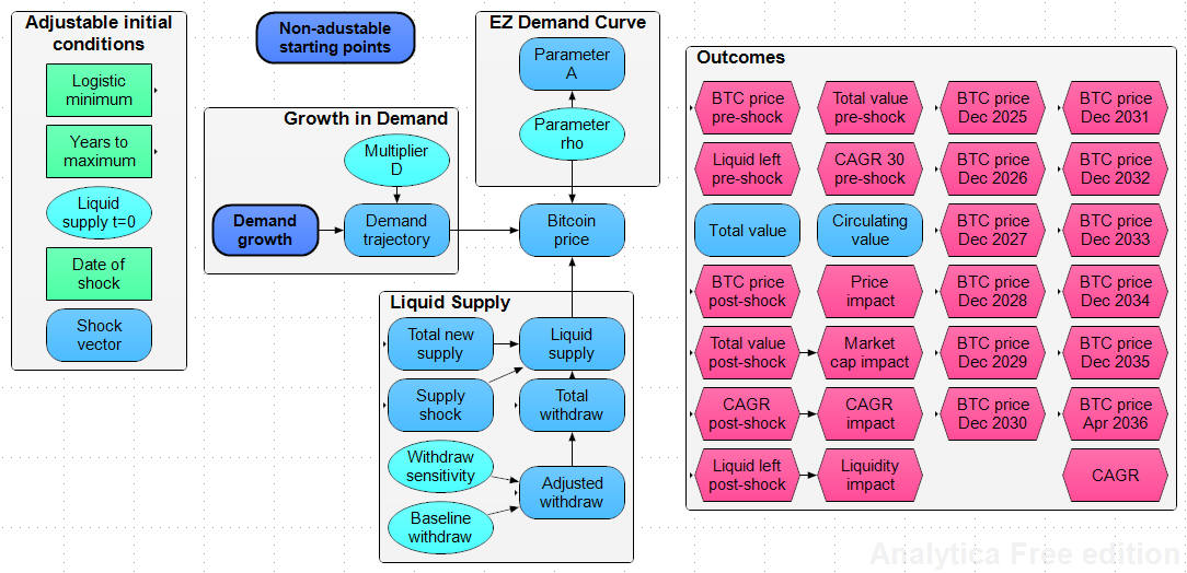
The model builds on the Epstein-Zin (EZ) recursive utility function, which separates investors' risk preferences from their willingness to shift purchases between today and the future. This is more realistic than simpler demand specifications because it allows the model to distinguish between momentum traders (who rebalance quickly as prices move) and long-term holders (who accumulate steadily regardless of short-term price action).

Price at each daily time step is calculated as:

P(t) = A'(t) x P0 x [(q0 - illiquid - satoshi) / liquid_supply(t)]^(1/rho)

where A'(t) is a logistic demand growth curve scaled by the demand multiplier, P0 is the starting price ($64,858 on April 20, 2024), and the ratio in brackets captures how shrinking liquid supply pushes price upward.

Parameters you can adjust

The interactive tool provides sliders for seven parameters, organized into four groups.

Initial supply

These settings determine how much Bitcoin is actually available for trading at the model's April 2024 start date. Total circulating supply was 19,687,500 BTC. From that, you subtract:

Satoshi coins (default: 968,000 BTC) -- Bitcoin attributed to Satoshi Nakamoto's early mining that has never moved and is presumed inaccessible.
Lost BTC (default: 1.57 million) -- Coins permanently lost due to forgotten keys, hardware failures, or deaths.
Illiquid BTC (default: 5.76 million) -- Bitcoin held long-term by investors with no near-term intention to sell. This is the most uncertain parameter. The model constrains the resulting initial liquid supply to between 1 million and 16.5 million BTC.

Adoption curve

These parameters shape how quickly Bitcoin demand grows over the model's time horizon:

T* (default: 14 years) -- The number of years until the adoption curve reaches saturation. Shorter values compress growth into fewer years, producing steeper price acceleration earlier. Longer values spread adoption more gradually.
L_min (default: 0.05) -- Controls the shape of the logistic S-curve. Values closer to zero produce a sharper inflection point (more sudden transition from slow to rapid adoption), while higher values produce a more gradual, nearly linear growth path.

Demand and preferences

D -- demand multiplier (default: 20) -- Scales the overall level of demand growth over the model's horizon. A value of 10 represents modest adoption growth; 100 represents aggressive institutional and sovereign accumulation. This is the single most important demand-side parameter.
rho -- EZ intertemporal substitution parameter (default: 2.0) -- Governs investors' willingness to shift purchases across time. Low values (0.5) represent fast, price-sensitive rebalancing typical of momentum traders. High values (2.5) represent patient, long-horizon accumulation typical of strategic reserve builders. Higher rho dampens short-run price spikes but supports sustained long-run appreciation.

Withdrawal behavior

q_base -- daily withdrawals (default: 2,000 BTC/day) -- The number of Bitcoin removed from liquid supply each day through institutional purchases, corporate treasury allocations, sovereign reserve building, and individual HODLing. Current evidence suggests 5,000-6,000 BTC per day are being removed. This parameter exerts the strongest influence on whether the model enters hyperbolic price territory.
alpha -- withdrawal sensitivity (default: 0.10) -- Controls how much rising prices throttle the rate of withdrawal. At alpha = 0, buyers purchase a fixed number of Bitcoin regardless of price. At alpha = 0.50, purchases are heavily curtailed as price rises (approximating a fixed dollar budget). This parameter acts as a behavioral brake on runaway price appreciation.

What to look for

The model produces five chart views:

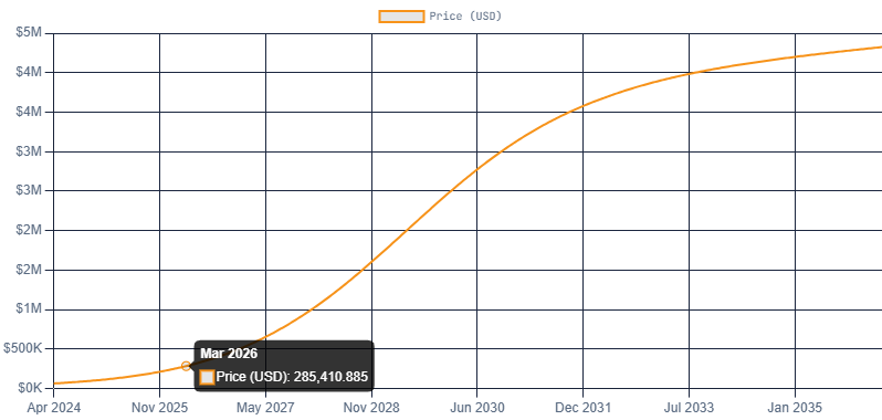
Price -- The forecast price trajectory, capped at $25 million to maintain visual clarity in hyperbolic scenarios.
Liquid supply -- How the tradeable Bitcoin pool shrinks over time. A red reference line marks 2 million BTC, the approximate threshold where hyperbolic price dynamics begin.
Supply flows -- Daily miner production (stepping down at each halving) versus daily reserve withdrawals (declining as the alpha sensitivity throttles purchases at higher prices).
Adoption curve -- The logistic adoption path (gamma) and the resulting demand shift parameter (A').
Price + Supply overlay -- Both trajectories on dual axes, making visible the inverse relationship between shrinking supply and rising price.

Summary statistics above the chart show the forecast April 2036 price, 12-year compound annual growth rate, total market capitalization, the date Bitcoin crosses $1 million, and final liquid supply.

Key findings from the research

Under baseline assumptions, the model projects Bitcoin prices in the low single-digit millions by the mid-2030s, consistent with a market capitalization in the $30-40 trillion range. The most important results:

Daily withdrawal rates above 5,000-6,000 BTC per day can push liquid supply below the 2 million threshold where hyperbolic price dynamics emerge.
Demand growth alone (even at D = 100) cannot trigger hyperbolic pricing if liquid supply remains above 6 million BTC.
The withdrawal sensitivity parameter (alpha) is the primary mechanism that prevents runaway prices -- it represents the real-world budget constraints that slow accumulation as Bitcoin becomes more expensive in fiat terms.
Hyperbolic outcomes are not inevitable. They concentrate in a specific region of parameter space: high withdrawal rates combined with low withdrawal sensitivity. The model helps locate exactly where right-tail risk lies.

Early lessons from the real world

Bitcoin price, currently around $70,000 as I write this, is substantially lower than model predictions. One of things that is possible with this model is to tweak parameter values to 'pessimistic' settings and see where we would be now if Bitcoin price was only just driven by current supply and demand parameters only.

For instance, try setting:

all 3 quantity values at 1 million each (very pessimistic for lost and illiquid coins). One lesson over the past year has certainly been that far more OGs than expected sold into what they viewed as end-of-cycle and industrial-scale Bitcoin miners have been selling as they pivot to AI high-performance compute.
T* = 16 yrs and L_min=0.08 (giving the slowest and flattest demand growth curve from the original parameter set). In a future model revision, I will also change the range of these parameters for more conservative options.
D=10 and rho=2.5 (the bottom end of the market demand shift parameter; and the highest time preference for 'traders' - rather than HODLers with low time preferences).
Q_base=1000 Bitcoin per day permanently to reserve (seems extremely conservative given ongoing withdrawals even my MSTR itself) and alpha to 0.25.

That combination of values gives us a March 2026 price prediction of $105.5k, and 16.165 million liquid supply.

Are those parameter values and outputs believable? Personally, I do not think we have anywhere near 16 million in available Bitcoin supply and that supply is being drained at a far higher rate than 1000 per day.

But our market price is 33% under the predicted price.

What else could cause this discrepancy? To me, it seems most plausible that financialization has dampened price appreciation. The flood of futures and options available in today's market functionally increases short-term supply so that there is a kink in the supply curve near market price (rather than a fixed vertical supply curve for any particular time period). So instead of 16 million of real liquid supply, perhaps we have a functional supply of 25 million, 30 million, or more Bitcoin in the marketplace when 'paper Bitcoin' is accounted for.

At some time, that issue will likely resolve itself and leverage will unwind.

But so far, I don't have a functional way to measure or incorporate the impacts of financialization into this model. I would love to do that - hope someone from an organization that could fund a research project might read this and reach out!

The interactive model runs entirely in your browser. No data is collected or transmitted. All computations occur client-side in JavaScript.

Exploring Bitcoin's Price Trajectory: An Interactive Supply-Demand Model

What this model does

The economic framework